3  The Power of Patchwork

We will combine a table and a plot into a single graphic, using the {patchwork} package. Let’s start by loading in some data from {medicaldata}

library(dplyr)

Attaching package: 'dplyr'

The following objects are masked from 'package:stats':

    filter, lag

The following objects are masked from 'package:base':

    intersect, setdiff, setequal, union

library(medicaldata)
library(gt)

We will now create a summary table in gt that compares radiographic outcomes by arm from 1 = Death to 6 = Considerable improvement. 3 = Moderate deterioration and 4 = No change

This HTML table would show up in RStudio in the Viewer tab.

d <- medicaldata::strep_tb 
d |> select(arm, rad_num) |> 
  group_by(arm) |> 
  summarize(rad6m = mean(rad_num),
            sd = sd(rad_num)) |> 
  gt::gt() ->t1
t1

arm	rad6m	sd
Control	3.134615	1.726709
Streptomycin	4.672727	1.732634

Now let’s convert this table into a gtable object composed of 11 grobs (graphical objects), which you can see in the Console. Notice that you now have to plot it to make it show up, amd in RStudio it would show up (by default) centered in the Plots tab.

library(gtable)
gt1 <- t1 |> as_gtable()
gt1

TableGrob (3 x 5) "layout": 11 grobs
    z     cells           name
1   1 (1-1,2-2) column_label_1
2   2 (1-1,3-3) column_label_2
3   3 (1-1,4-4) column_label_3
4   4 (2-2,2-2)    body_cell_1
5   5 (2-2,3-3)    body_cell_2
6   6 (2-2,4-4)    body_cell_3
7   7 (3-3,2-2)    body_cell_4
8   8 (3-3,3-3)    body_cell_5
9   9 (3-3,4-4)    body_cell_6
10 10 (2-3,2-4)     table_body
11 11 (1-3,2-4)          table
                                 grob
1   gt_grid_cell[GRID.gt_grid_cell.3]
2   gt_grid_cell[GRID.gt_grid_cell.6]
3   gt_grid_cell[GRID.gt_grid_cell.9]
4  gt_grid_cell[GRID.gt_grid_cell.13]
5  gt_grid_cell[GRID.gt_grid_cell.17]
6  gt_grid_cell[GRID.gt_grid_cell.21]
7  gt_grid_cell[GRID.gt_grid_cell.25]
8  gt_grid_cell[GRID.gt_grid_cell.29]
9  gt_grid_cell[GRID.gt_grid_cell.33]
10 gt_grid_cell[GRID.gt_grid_cell.36]
11 gt_grid_cell[GRID.gt_grid_cell.39]

plot(gt1)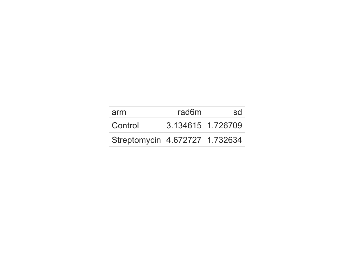

Now we will make our plot, which will show up in RStudio in the Plots tab. Run the code below to get the plot. We use expand_limits in ggplot to make extra room for the table. The Streptomycin column is 1, and the Control column is 2. We are expanding to add empty columns 3 and 4. Run the code with the blue Run Code button, then Turn off expand_limits with a hashtag to comment it out to see how this works, then Run the code again. Do you know what would happen if we used geom_point? Try it out in the code chunk below. Re-run the code. Click on the Start Over button to restore the code to its original state.

Now insert the gt1 graphical object table into the plot with the {patchwork} function, inset_element, using the code below at line 25 and beyond. The first 23 lines rebuild the table and plot objects. Run the code. The standard ggplot has the point 0,0 at bottom left, and the point 1,1 at the top right. In the last part of the code chunk below, experiment with the location of the plot by changing the TRBL (pronounced ‘trouble’) parameters, then rerun the code. Also experiment with the alignment - options include ‘full’ and ‘plot’, and run the code, to see if you can figure out what the table is being aligned with for each option.